Introduction

In simple terms, normalization is a way to improve the quantitative accuracy of Western blot data by correcting for small lane-to-lane and sample-to-sample variation. Several normalization methods are available, but the goal of each is to correct for variability inherent to Western blotting. No single normalization method can correct for everything. However, when used properly, normalization can minimize many common sources of variation, such as:

• Uneven sample loading

• Load volume

• Irregularities across the blot due to problems such as inconsistent transfer, uneven blocking, or uneven antibody incubation

What You Will Learn from This Guide

This guide will present examples where normalization has been adversely affected by common pitfalls and will offer potential solutions.

Inaccurate normalization has many causes, including:

1. Incorrect experimental design

2. Improper experimental technique

3. Misuse of software tools

Normalization Basics

Normalization mathematically corrects for unavoidable sample-to-sample and lane-to-lane variation by comparing the target protein to an internal loading control.

The target and internal loading control must be detected within the same linear range.

1. Internal loading control (ILC): Endogenous protein(s) that are unaffected by experimental conditions and used as an indicator of sample loading (11).

   Several types of ILC can be used, including:

   • An unrelated internal reference protein, typically a housekeeping protein (HKP, such as actin, tubulin, or GAPDH) that is expressed in all samples at a stable, constant level.
   • Total protein staining of the membrane after transfer to visualize actual sample loading in each lane.

2. Linear range (LR): The span of signal intensities that display a linear relationship between amount of protein on the membrane and signal intensity recorded by the detector.

Accurate normalization requires that the target and internal loading control signals are both entirely dependent on sample loading.

Normalization Requirements

For a normalization strategy to be accurate, it must conform to the core principle of normalization. To ensure that your strategy is accurate, verify that your ILC meets these requirements:

1. The ILC must be unaffected by experimental conditions.

2. The ILC and target must be detected within the same linear range.

3. The ILC must not interfere with target detection.

Choosing and validating an ILC that meets these requirements is fundamental to the design and accuracy of a quantitative Western blot.

The Normalization Handbook (licorbio.com/handbook) describes how to choose and validate an appropriate internal loading control.

This guide focuses on examples of how normalization can go wrong, and provides tips for avoiding such problems.

Experimental Design

Small sample-to-sample and lane-to-lane variations are inevitable. However, a well-designed protocol will reduce the impact of this inherent variation on your results. Examples in this section will show why the following points are important to consider when you plan an experiment.

1. Ensure even sample loading: Differences between protein abundance on a blot cannot be determined unless the same amount of sample protein is loaded in each lane. To ensure each sample begins with the same amount of protein, a protein concentration assay must be used to adjust sample concentration and make sample loading across your gel as consistent as possible.

2. Normalize: An accurate normalization strategy can correct for minor variation that occurs in spite of careful experimental technique. Your internal loading control and target must vary to the same degree with sample loading for normalization to be accurate.

3. Replicate, replicate, replicate: Even with consistent sample loading and accurate normalization, replication is still necessary. Technical replicates will help you identify inaccuracies caused by processing variability.

Total Protein Staining Is a Reliable Indicator of Sample Loading

Your ILC must provide a reliable readout of sample loading, or normalization will not be accurate. Total protein staining (TPS) of membranes is one type of ILC that can provide a robust, reliable readout of sample concentration. TPS is emerging as the new standard method for Western blot normalization (11). The Journal of Biological Chemistry explicitly recommends this method, stating in the "Instructions For Authors" that the journal would:

"prefer that signal intensities are normalized to total protein by staining membranes with Coomassie Blue, Ponceau S, or other protein stains.” (Journal of Biological Chemistry, "Instructions for Authors.” The Journal of Biological Chemistry. American Society for Biochemistry and Molecular Biology. Web. 3 March 2016.http://www.jbc.org/site/misc/ifora.xhtml#blots)

After transfer, the membrane is treated with a total protein stain to assess actual sample loading across the blot. Because total protein staining uses the combined readout of many different sample proteins in each lane, error and variability are minimized. Total protein staining is also used to monitor and confirm protein transfer across the entire blot, at all molecular weights.

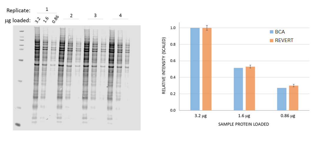
Revert™ 700 Total Protein Stain is a near-infrared fluorescent membrane stain that can be imaged at 700 nm with an Odyssey^® imaging system. Revert staining is used to normalize your target protein to the total amount of sample protein present in each lane. Fluorescent signal from stained membranes is proportional to the amount of total sample protein loaded (see Figure 74).

For more information about Revert™ 700 Total Protein Stain, see licorbio.com/revert.

Revert Staining Is Highly Correlated with Sample Loading

Figure 74 demonstrates that Revert staining is proportional to total sample protein. In this experiment, total protein concentration of samples was quantified by the bicinchoninic acid (BCA) assay, and gels were loaded uniformly with equivalent amounts of sample protein. After electrophoresis and transfer, the membrane was stained with Revert 700 Total Protein Stain. The relative difference between known load amount and stained protein signal was then compared to examine the correlation between Revert staining and sample protein loading as determined by BCA.

Total Protein Loading: An Emerging Alternative for Normalization

Recent studies point to total protein detection as the emerging “gold standard” for normalization of protein loading. In this method, the membrane is treated with a total protein stain to assess sample loading in each lane, prior to immunoblot analysis. Many reference points are combined, reducing the impact of biological variability on quantification.

The Journal of Biological Chemistry now explicitly recommends normalization to total protein loading, stating that “we prefer that signal intensities are normalized to total protein by staining membranes with Coomassie Blue, Ponceau S, or other protein stains ("Instructions for Authors.” The Journal of Biological Chemistry. American Society for Biochemistry and Molecular Biology. Web. 3 March 2016.http://www.jbc.org/site/misc/ifora.xhtml#blots).”

Total protein loading is typically assessed by staining of the membrane after transfer (4, 11, 31, 32). Staining must be compatible with downstream immunodetection and should not alter or damage sample proteins. Some total protein methods, such as the Stain-Free trihalo labeling technology, rely on covalent labeling of sample proteins for detection (23, 33, 4). However, membrane staining may be a more versatile approach, because it requires minimal alteration of Western blot protocols and bypasses the concerns raised by irreversible covalent modification of sample proteins (23, 33, 4).

Recent studies indicate that one of the most common methods may sometimes be unreliable – and publication standards are becoming more stringent. For these common HKPs, stable protein levels are generally assumed. However, an increasing number of gene expression and protein expression studies indicate that expression may be less stable than believed (10).

Estimate Total Protein Concentration Before Loading Gel

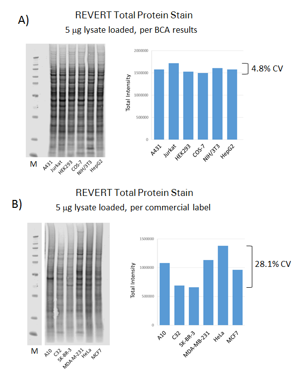
Each lane must be uniformly loaded with an equivalent amount of total sample protein. A protein concentration assay must be used to adjust sample concentration and make sample loading as consistent as possible. The experiment in Figure 75 shows the importance of estimating protein concentration.

First, samples were adjusted for uniform loading based on either BCA measurements or the manufacturer's labeled concentration. Revert™ 700 Total Protein Stain was then used to compare the total sample protein between lanes.

Total protein staining was very consistent for lysates loaded according to empirically-measured concentration, even though the samples were from very different sources: A431 – Hu epidermis, Jurkat – Hu blood, HEK293 – Hu kidney, COS-7 – Monkey kidney, NIH/3T3 – Mouse fibroblast, HepG2 – Hu liver.

In contrast, lysates loaded according to the labeled concentration showed considerable variation in total protein staining. This underscores the importance of empirically verifying protein concentration to ensure consistent sample loading.

Replicates for Statistical Analysis

Both biological and technical replicates are necessary for accurate and reliable results.

• Biological replicate: parallel measurements of biologically distinct samples that capture random biological variation, which may itself be a subject of study or a source of noise (30).
• Technical replicate: repeated measurements of the same sample that represent independent measures of the random noise associated with protocols or equipment (30).

In addition to replicate blots, replicate sample lanes should be included within a blot. Replicate sample lanes help you characterize intra-blot variability, to verify that observed changes in band intensity are above the error of measurement and background threshold.

Technical replicates can expose some common sources of variation.

Sample Loading

Inconsistent sample loading cannot be avoided entirely. However, variation can be identified by running replicate blots and/or lanes. Visual assessment of membranes is helpful in spotting variation, but appearances can be misleading. Quantification of bands should be used for more definitive answers. Normalization must be used to minimize the impact of variation.

Inconsistent sample loading can affect data analysis, as seen in Figure 76. In this experiment, phospho-ERK was detected in an A431 cell lysate. The sample was loaded in triplicate. To mimic variation in sample loading, material from lane 1 was allowed to leak into the adjacent sample lane. After electrophoresis and transfer, Revert™ 700 Total Protein Stain was used to visualize total sample protein on the blot, followed by NIR fluorescence immunoblotting to detect p-ERK. Sample leakage caused a large coefficient of variation (CV) in raw p-ERK signals in the replicate lanes. Data were then normalized to total protein staining, to correct for inconsistent sample loading. After normalization, the CV for p-ERK was reduced by 130%.

Membrane Transfer

Replicates are also important for spotting variation that may be caused by transfer. The transfer process introduces many possible sources of variation:

• Transfer stack position in the tank
• Loading position on the gel
• Inconsistent temperature across the membrane
• Inconsistent electric field across the membrane
• Improperly prepared transfer stack

The following example shows variation caused by an improperly prepared transfer stack. Although transfer variation can be spotted visually in this example, visual assessment can be misleading. Bands should be quantified for definitive answers.

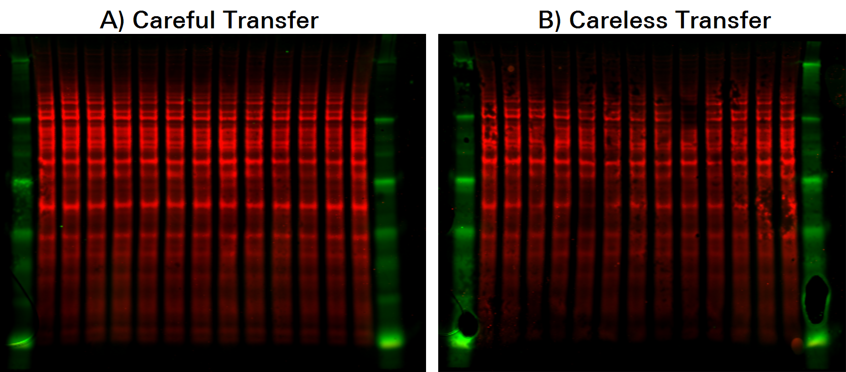
Further, total protein staining makes it possible to monitor transfer consistency across the entire blot at all molecular weights. This will help you spot any irregularities that might indicate the experiment should be repeated.

For more tips on improving your transfer, refer to the Protein Electrotransfer Tech Note (licorbio.com/proteintransfer).

Stripping and Reprobing

Although stripping and reprobing is common, it’s also time-consuming and will introduce variability into your analysis and normalization procedure. To improve accuracy and precision, replicate blots can be performed, but two-color fluorescence is the most accurate alternative to stripping and reprobing.

• If stripping is incomplete, residual antibody will generate artifacts when the blot is reprobed. This is particularly problematic if the two proteins co-migrate. In addition, complete removal of bound antibodies may be difficult to achieve.
• Stripping can damage or wash away target protein. It may also cause significant loss of sample proteins from the membrane, perhaps 25% or more of the target in a single stripping cycle (4, 16).

Outcomes from various stripping conditions were examined in a 2015 study, using immunoblots probed with p-ERK1/2 antibody and a GAPDH internal control (3).

• Low pH Glycine Buffer Solution: Low-pH glycine stripping was very ineffective, with considerable residual antibody staining for p-ERK1/2 and GAPDH.
• Guanidinium stripping: Although more effective for removal of GAPDH antibody, a p-ERK1/2 artifact remained.
• SDS stripping with β-mercaptoethanol: This removed the GAPDH and p-ERK1/2 antibodies, but caused substantial loss of total protein from the membrane.

• Janes describes stripping and reprobing as a “quantitative trade-off between antibody removal and total protein loss” (3). Protein-specific factors such as membrane saturation, amino acid composition, and post-translational modification are other potential areas of concern.
• Multiplex fluorescent immunoblotting makes normalization with an internal control simpler, more convenient, and more accurate. The blot is incubated with primary antibodies raised in different hosts. Secondary antibodies labeled with spectrally-distinct fluorescent dyes are then used to simultaneously detect the internal control on the same blot and in the same lanes as the target protein (26, 27). Blots are digitally imaged to detect the stable fluorescent signals. Stripping is not required, co-migrating proteins can be detected, and antibody cross-reactivity is easily identified.

Housekeeping Proteins

Normalization relies on an ILC to minimize the impact of sample-to-sample variation on your quantitative Western blot data. However, if your ILC is affected by the experimental conditions, it can actually introduce variability. HKPs are widely used for Western blot normalization, and stable levels of these proteins are generally assumed. However, recent studies indicate that HKP levels may be less stable than previously believed (10). Because HKP normalization is based on a single internal reference protein, unexpected or unnoticed changes in expression of this HKP alter the interpretation of the sample loading indicator. This source of error will affect quantitative analysis and limit your ability to detect actual changes in your samples.

The Normalization Handbook (licorbio.com/handbook) explains the HKP normalization strategy, and provides a procedure for validating a HKP for normalization.

Verify That HKP Expression Is Not Affected by Treatment

Before using a housekeeping protein for normalization, you must validate that its expression is constant across all samples and is unaffected by your specific experimental context and conditions. Empirical validation is becoming more common in the literature, and may be required by some publishers. New submission guidelines for Western blot data from the Journal of Biological Chemistry “strongly caution against the use of housekeeping proteins for normalization, unless there is a clear demonstration that expression of the housekeeping protein is unaffected by the experimental treatments” ("Instructions for Authors.” The Journal of Biological Chemistry. American Society for Biochemistry and Molecular Biology. Web. 3 March 2016.http://www.jbc.org/site/misc/ifora.xhtml#blots).

HKP levels can be affected by experimental manipulations

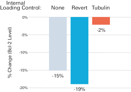
Figure 78 demonstrates the possible impact on data analysis and interpretation if an HKP with variable expression is used for Western blot normalization. Bcl-2 levels were examined in Jurkat cells, before and after treatment with etoposide, a topoisomerase inhibitor. Levels of Bcl-2 and tubulin (HKP used as ILC) were analyzed by multiplex fluorescent Western blotting. Bcl-2 signals were then normalized to either tubulin or Revert™ 700 Total Protein Stain.

Before normalization, raw Bcl-2 signals indicated a 15% decrease in abundance of Bcl-2 after etoposide treatment (Figure 78). Normalization to total protein staining resulted in a 19% measured decrease in Bcl-2. However, normalization to tubulin yielded a very different result: a small decrease of only 2% in Bcl-2 expression that may not be statistically significant. Validation experiments revealed that tubulin expression was affected by this experimental treatment (tubulin level was 16% lower in etoposide-treated samples than untreated samples). This experiment indicates that an HKP with variable expression can alter the interpretation of experimental results, potentially concealing biologically relevant differences between samples.

Treatment Conditions Known to Affect HKP Expression

Many treatment conditions can affect HKP expression (4 - 15), including:

• Experimental manipulation (such as temperature, cell confluence, or drug treatments)
• Tissue type
• Cell line
• Age of culture
• Disease or injury state

Odyssey Loading Indicator

The Odyssey Loading Indicator (OLI), a 28 kDa recombinant protein directly labeled with near-infrared fluorescent dyes, can be used as part of the process to determine if the HKP is stably expressed. Since OLI is exogenous, it is unaffected by up or down regulation caused by experimental treatment. When you detect OLI and the HKP simultaneously, the difference in their respective signals can be used as part of the process to determine if the HKP is stably expressed or not.

Accurate normalization relies on an internal loading control, an endogenous protein used as an indicator of sample concentration. Since the OLI is an exogenous protein, it functions as an external loading control, and cannot be used for normalization.

Verify that HKP can be detected with linear range of target

Many target proteins are low-abundance compared with ubiquitous HKP and structural proteins (11). If your target is low-abundance but your HKP is highly abundant, the two proteins will produce bands with very different intensities.

If the target bands are faint but the HKP bands are strong, it may be difficult to detect your HKP and target within the same linear range. Outside the linear range, the relationship between protein and measured signal is unknown. The target and ILC signal will not vary to the same degree with sample loading, so the Core Normalization Principle will not hold. Normalization accuracy could be affected.

In addition, the strong HKP band may become saturated, which means it cannot be quantified or used for normalization.

Revert™ 700 Total Protein Stain

The Revert 700 Total Protein Stain is a membrane stain used to normalize target protein to the total amount of sample protein per lane. Revert 700 Total Protein Stain fluoresces at 700 nm, and signal from Revert staining is proportional to sample loading.

Please see licorbio.com/revert for more information about Revert 700 Total Protein Stain.

With a total protein stain, you can monitor protein transfer across the entire blot at all molecular weights. This will allow you to determine if there are any irregularities that indicate you should run the blot again to get more robust results.

Revert™ 700 Total Protein StainFrequently Asked Questions

Should I stain my Western blot membrane with Revert 700 Total Protein Stain before or after I dry the membrane?

You can use Revert 700 Total Protein Stain on a membrane that was kept wet or dry following transfer. To use on a dry membrane, briefly wet the membrane in water prior to adding the Stain Solution. For PVDF membranes, rinse first in methanol, followed by water.

Can I reuse Revert 700 Total Protein Stain?

Revert 700 Total Protein Stain is intended for a single use and reusing the stain on additional membranes is not recommended. Reusing the stain will affect normalization accuracy.

Will Revert 700 Total Protein Stain work with the iBind?

Yes, Revert 700 Total Protein Stain is compatible with the iBind and nitrocellulose membranes.

If you use PVDF membranes, you may need to optimize your procedure to ensure a low membrane background. Increasing the time for your wash steps may lower the background.

Does Revert 700 Total Protein Stain interfere with antibody binding or the detection of my Western blot target?

Revert 700 Total Protein Stain is compatible with all subsequent Western blot immunodetection procedures and does not interfere with antibody binding.

How sensitive is Revert 700 Total Protein Stain?

Revert 700 Total Protein Stain is intended for staining total protein in individual lanes and has a linear detection range of 1-60 µg when used with cell lysate. However, individual proteins are easily detectable at low nanogram amounts.

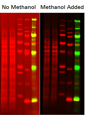
After staining my membrane with Revert 700 Total Protein Stain, I am not seeing any band development.

Here are some possible causes:

• Transfer was compromised. Check to see if your molecular weight ladders transferred.
• Membrane was not rinsed with water prior to staining.
• Methanol was not added to the Stain Solution.

Do you have any tips for lowering membrane background after staining with Revert 700 Total Protein Stain?

Be sure to add 30 mL of methanol to the Stain Solution prior to use (as described in the protocol).

How should I store Revert™ 700 Total Protein Stain and what is the shelf life?

We recommend storing Revert 700 Total Protein Stain at room temperature where it is stable for 6 months from the date of receipt.

Can I strip and reprobe Western blots stained with Revert 700 Total Protein Stain?

Yes, you can strip and reprobe the membrane for subsequent detection of another target in the 800 nm channel. However, stripping and reprobing introduces random variation into your experiment. Blots that have been stripped and reprobed should not be quantified. See Stripping and Reprobing for more information.

Can I use Revert 700 Total Protein Stain on a blot that was stripped?

The signal will be weak, so we do not recommend using the Revert 700 Total Protein Stain signal to normalize the reprobed target.

Can I stain my blot with Revert 700 Total Protein Stain after blocking the membrane?

No, Revert 700 Total Protein Stain will also stain blocking buffer proteins that bind to the membrane. This increases membrane background and significantly interferes with accurate detection.

Can Revert 700 Total Protein Stain be detected by other imagers?

For the best results, use Odyssey Imaging Systems, which are designed for superior near-infrared detection. Other imagers capable of detecting signals in the 700 nm channel can also be used with the stain. Alternatively, white light imagers can detect Revert 700 Total Protein Stain. However, the linear and dynamic range will be reduced.

Detection Methods Have Different Linear Ranges

For accurate quantitation and normalization, your detection method must have sufficient linear range to capture the brightest and faintest signals from your blot. Choose a detection method that works for your normalization strategy.

Linear Range Definition

Outside the linear range of detection, the relationship between the amount of protein on the blot and the measured signal is unknown. Protein levels cannot be quantified outside the linear range, so you must ensure your ILC and target can both be detected within the same linear range.

Linear range is an especially important consideration if you plan to use a housekeeping protein (HKP) for normalization. Many frequently studied target proteins are low-abundance compared to ubiquitous HKPs (11), making it difficult to detect the target and HKP in the same linear range.

If your target is low abundance, it is likely that you will need to load a large amount of sample to detect it. However, loading a large amount of sample will cause a highly-abundant HKP band to produce a bright signal that is outside the linear range of the target. The HKP band may even reach saturation, meaning the signal is too bright to be recorded by the detection system and is unquantifiable. The HKP signal cannot be used for normalization if it is saturated or outside the linear range of the target.

See the Normalization Handbook (licorbio.com/handbook) to learn more about how to ensure your normalization strategy is not affected by the linear range of your system.

Detection Method Linear Range

The linear range of your imaging system is a key factor in determining if your loading control and target can be detected in the same linear range. Film has an extremely narrow linear range. Due to the physical basis of how film records signal, film is disproportionately insensitive to signal at both high (18, 19) and low intensities of light (18). Even some CCD imagers are prone to signal saturation.

This section provides a comparison of several detection systems, and shows an example of saturation on film.

Detection Method Comparison

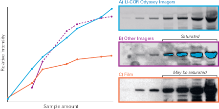
Film Saturation

Although saturation can occur on some digital systems, film is particularly prone to saturation. Film records signal through the use of silver grains that are activated in response to light. Saturation occurs on film when the finite number of silver grains in a region of the film have all been activated, meaning no more light can be detected.

In addition, film becomes progressively less responsive to light as it nears saturation. As more silver grains are activated by photons, it becomes statistically less likely that each new photon will strike a grain that has not already been activated (18 - 19). Photons that do not activate silver grains will not be recorded as signal.

Software Analysis

Normalization cannot correct for inaccuracy or inconsistency in software analysis. For accurate quantitative Western blot data, ensure you are using your software analysis tool correctly and according to the instructions.

The following section will show best practices for using Image Studio to attain consistent results, and some ways variability can be introduced into your analysis using other software packages.

Define the Region of Interest (Shape) Accurately

Ensure the regions of interest (shapes) used to define the protein bands you are interested in quantifying are defined correctly.

View a Shape's Pixel Intensity Profile to Accurately Define Shape

In Image Studio, the Profiles tab allows you to see if your shapes have been drawn correctly around bands. If you select a shape, the Shape profile shown in the Profiles tab should look similar to (Figure 82).

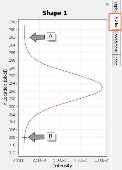
Using the Profiles Tab To See If a Shape Overlaps Multiple Bands

Only one peak should appear in the shape profile if only one band is enclosed by the shape and the shape's background border.

In Figure 1, the background border width is set to 2 pixels and only one band is enclosed by Shape 1, so one peak appears in the Profiles tab. When the background border for Shape 1 is increased to 5 pixels (see Figure 2), the border can be seen to overlap another shape and an extra peak begins to appear in the Profiles tab.

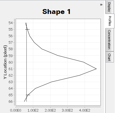
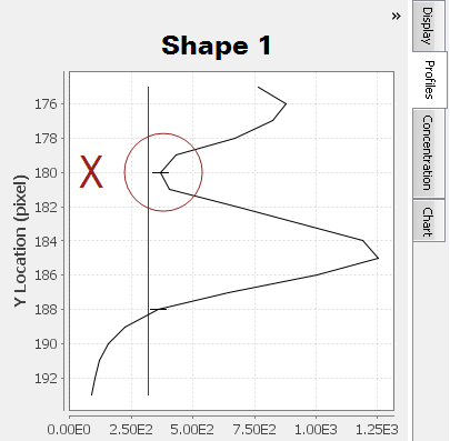
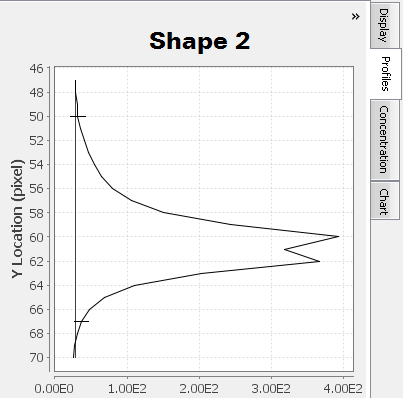
Multiple "humps" may exist at the top of a peak . Carefully examine the Profiles tab in conjunction with the background border surrounding the shape to ensure multiple "humps" are from the same band and not different bands. For Shape 2, a less dense area inside the band is causing two peaks to appear in the Profiles tab.

Background Subtraction

Background must be subtracted to accurately calculate signal from the regions of interest, especially if background values vary throughout an image. The best method for background correction depends on the image and the consistency of its background levels.

Many background subtraction methods are available.

Image Studio Lane vs ImageJ Rolling Ball

The Image Studio Lane background subtraction method and the Rolling ball method available in ImageJ use very different algorithms to subtract background from a lane. Rolling ball can also be used to subtract background from an entire image, although this will alter the underlying image data.

Using Rolling ball to subtract background from an entire image is discouraged (25).

The Image Studio Lane background subtraction method is available with the Western Analysis Key (see licorbio.com/AnalysisKeys for more information).

Image Studio Lane Background Subtraction

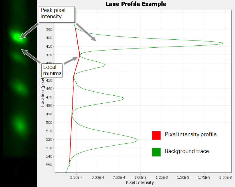
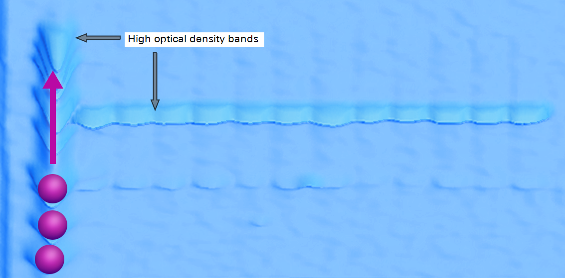
To begin the Image Studio Lane background subtraction algorithm, the average pixel intensity of each row of pixels in a lane is calculated to establish a "lane profile". The lane profile is used to find areas of minimum pixel intensity between shapes, called "local minima". Figure 86 shows a lane with its corresponding lane profile.

To subtract background, a linear connection is drawn between consecutive local minima and background noise that falls beneath the lines is subtracted. The Lane background subtraction method accurately subtracts background without being affected by shape size, shape spacing, or image resolution.

A full description of the Lane background subtraction algorithm is available in the help (licorbio.com/BgSubtractHelp).

ImageJ Rolling Ball Background Subtraction

Rolling ball can be applied to an entire image, although this practice is discouraged (25).

To understand Rolling ball, imagine an image of a Western blot as a 3-dimensional histogram of pixel intensity (Figure 87). Shapes, areas of high pixel intensity, will be peaks on the histogram.

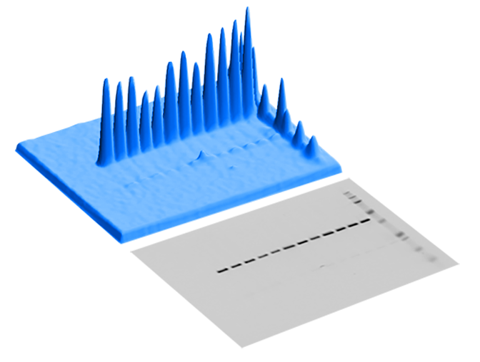
Rolling ball identifies background in an image by traversing a ball along the bottom surface of the pixel intensity histogram. The highest point where the ball can fit underneath the surface is considered the threshold for background subtraction at that point (Figure 88).

Differences between Rolling Ball and Lane

Image Studio Lane and ImageJ Rolling ball are different in two key ways.

1. Rolling ball requires a user to choose a radius that will be used for background subtraction. Lane does not require input to accurately subtract background.

2. Rolling ball can be used to subtract background from an entire image, which will modify the underlying image data. Lane background can only be applied to a lane, and the background subtraction process does not change the underlying image data.

Whether Rolling ball is applied to an entire image or a lane, an appropriate radius must be chosen for accurate results. The correct radius is dependent on many factors: image resolution, shape width, shape separation, and shape overlap. These factors are likely to vary throughout an image, so choosing a radius that allows for consistent, accurate background subtraction can be difficult.

When deciding if Rolling ball is appropriate for your analysis, consider the description of Rolling ball from the ImageJ documentation:

“Removes smooth continuous backgrounds from gels and other images” (28)

If the background does not appear smooth and continuous, another approach may be necessary for accurate quantification and normalization.

ImageJ Manual Background Subtraction

Another option for analyzing Western blots in ImageJ is to use the Gel analysis to plot a profile of a band or lane. The background can be drawn manually using the Segment tool and peaks can be selected manually using the Magic Wand tool.

Since the background is determined manually and subjectively in this workflow, the analysis is open to variability.

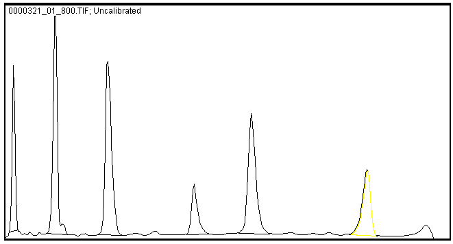
Image Format

Do not quantify lossy format images, such as JPEGs.

Some image types undergo a software process known as “compression” when they are saved. This process makes the file size smaller, but it also results in irreversible data loss. To ensure you are analyzing the best available data, do not analyze lossy images, such as JPEGs.

Image Studio Software saves scans to 16 bit TIFF images. Only the original 16 bit TIFF files should be used for analysis. If you need to move Image Studio images between computers, use the export Zip File option.

Data Loss from Scanning

In addition to the fact that film can only record data within a narrow linear range, further data loss can be caused by digitizing film on an office scanner. Gassman et. al. compared images acquired on a CCD with images acquired by scanning film, and the scanned image was found to have a 2.6 times lower dynamic range (25).

Data loss caused by scanning can lead to inaccurate quantification and normalization.

Summary

Consistent and accurate quantitative immunoblotting relies on keeping error to a minimum and normalizing for the error that will inevitably occur.

References

1. "Instructions for Authors.” The Journal of Biological Chemistry. American Society for Biochemistry and Molecular Biology. Web. 3 March 2016.http://www.jbc.org/site/misc/ifora.xhtml#blots

2. COX IV as a Loading Control licorbio.com/coxiv

3. Janes KA (2015) An analysis of critical factors for quantitative immunoblotting. Sci Signaling 8(371): rs2.

4. Gomes R, Gilda JE and Gomes AV (2014) The necessity of and strategies for improving confidence in the accuracy of Western blots. Expert Reviews Proteomics 11(5): 549-60.

5. Li X, Bai H, Wang X, Li L, Cao Y, Wei J, Liu Y, Liu L, Gong X, Wu L, Liu S, and Liu G (2011) Identification and validation of rice reference proteins for Western blotting. J Exper Biol. doi: 10.1093/jxb/err084.

6. Eaton SL, Roche SL, Llavero Hurtado M, Oldknow KJ, Farquharson C, Gillingwater TH, and Wishart TM (2013) Total protein analysis as a reliable loading control for quantitative fluorescent Western blotting. PLoS ONE 8(8): e72457.

7. Rocha-Martins M, Njaine B, Silveira MS (2012) Avoiding pitfalls of internal controls: validation of reference genes for analysis by qRT-PCR and Western blot throughout rat retinal development. PLoS ONE 7(8): e43028.

8. Pérez-Pérez R, López JA, García-Santos E, Camafeita E, Gómez-Serrano M, Ortega-Delgado FJ, et al. (2012) Uncovering suitable reference proteins for expression studies in human adipose tissue with relevance to obesity. PLoS ONE 7(1): e30326.

9. Prokopec SD, Watson JD, Pohjanvirta R, and Boutros PC (2014) Identification of Reference Proteins for Western Blot Analyses in Mouse Model Systems of 2,3,7,8-Tetrachlorodibenzo-P-Dioxin (TCDD) Toxicity. PLoS ONE 9(10): e110730.

10. Li R and Shen Y (2013) An old method facing a new challenge: re-visiting housekeeping proteins as internal reference control for neuroscience research. Life Sciences 92: 747-51.

11. Aldridge GM, Podrebarac DM, Greenough WT, and Waller IJ (2008) The use of total protein stains as loading controls: an alternative to high-abundance single protein controls in semi-quantitative immunoblotting.J Neurosci Meth 172(2): 250-54.

12. Greer S, Honeywell R, Geletu M, Arulanandam R, and Raptis L (2010) Housekeeping genes: expression levels may change with density of cultured cells. J Immunol Meth. 355(1-2): 76-9.

13. Lanoix D, St-Pierre J, Lacasse A-A, Viau M, Lafond J, Vaillancourt C. (2012) Stability of reference proteins in human placenta: General protein stains are the benchmark. Placenta 33: 151–156.

14. Yu HR, Kuo HC, Huang HC, Huang LT, Tain YL, Chen CC, et al. (2011) Glyceraldehyde-3-phosphate dehydrogenase is a reliable internal control in western blot analysis of leukocyte subpopulations from children. Anal Biochem 413(1): 24–9.

15. Barber RD, Harmer DW, Coleman RA, Clark BJ. (2005) GAPDH as a housekeeping gene: analysis of GAPDH mRNA expression in a panel of 72 human tissues. Physiol Genomics 21(3): 389-95.

16. Riis P (2001) Molecular Biology Problem Solver: A Laboratory Guide, edited by AS Gerstein. Wiley-Liss, Inc. Chapter 13: 373-97.

17. Bakkenist CJ, Czambel RK, Hershberger PA, Tawbi H, Beumer JH, Schmitz JC (2015) A quasi-quantitative dual multiplexed immunoblot method to simultaneously analyze ATM and H2AX Phosphorylation in human peripheral blood mononuclear cells. Oncoscience 2(5): 542–554.

18. Laskey, R.A. Efficient detection of biomolecules by autoradiography, fluorography or chemiluminescence. Methods of detecting biomolecules by autoradiography, fluorography and chemiluminescence. Amersham Life Sci. Review 23:Part II (1993).

19. Baskin, DG and WL Stahl. Fundamentals of quantitative autoradiography by computer densitometry for in situ hybridization, with emphasis on ³³P. J Histochem and Cytochem 41(12):1767-76 (1993).

20. Canetta SE, Luca E, Pertot E, Role LW, Talmage DA (2011) Type III Nrg1 back signaling enhances functional TRPV1 along sensory axons contributing to basal and inflammatory thermal pain sensation. PLoS ONE 6(9): e25108.

21. Meiler E, Nieto-Pelegrín E, Martinez-Quiles N (2012) Cortactin Tyrosine Phosphorylation Promotes Its Deacetylation and Inhibits Cell Spreading. PLoS One 7(3): e33662.

22. Gebhart C, Ielmini MV, Reiz B, Price NL, Aas FE, Koomey M, Feldman MF (2012) Characterization of exogenous bacterial oligosaccharyltransferases in Escherichia coli reveals the potential for O-linked protein glycosylation in Vibrio cholerae and Burkholderia thailandensis. Glycobiology 22(7):962-74.

23. Taylor SC and Posch A (2014) The design of a quantitative Western blot experiment. BioMed Res Intl. doi: 10.1155/2014/361590.

24. Degasperi A, Birtwistle MR, Volinsky N, Rauch J, Kolch W, Kholodenko BN (2014) Evaluating strategies to normalise biological replicates of Western blot data. PLoS ONE 9(1): e87293.

25. Gassmann M, Grenacher B, Rohde B, Vogel J (2009) Quantifying Western blots: pitfalls of densitometry 30(11):1845-55.

26. Schutz-Geschwender A, Zhang Y, Holt T, McDermitt D, and Olive DM (2004) Quantitative, two-color Western blot detection with infrared fluorescence. LI-COR Biosciences: 1-7.

27. Gerk PM (2011) Quantitative immunofluorescent blotting of the Multidrug Resistance-associated Protein 2 (MRP2). J Pharm Toxicol Methods 63(3): 279-82.

28. Subtract Background. ImageJ User Guide Section 29.14.

29. Rasband, W.S., ImageJ, U. S. National Institutes of Health, Bethesda, Maryland, USA, http://imagej.nih.gov/ij/, 1997-2016.

30. P Blainey, Krzywinski M, and Altman N (2014) Points of Significance: Replication Nature Methods doi:10.1038/nmeth.3091

31. Collins MA, An J, Peller D, and Bowser R (2015) Total protein is an effective loading control for cerebrospinal fluid western blots. J Neurosci Methods 251: 72-82.

32. Romero-Calvo I, Ocón B, Martinez-Moya P, Suárez MD, Zarzuelo A, Martinez-Augustin O, de Median FS (2010)Reversible Ponceau staining as a loading control alternative to actin in Western blots. Anal Biochem 401(2): 318-20.

33. Taylor SC, Berkelman T, Yadav G, and Hammond M (2013) A defined methodology for reliable quantification of Western blot data. Mol Biotechnol. 55: 217-226.