Housekeeping Protein Normalization Protocol

Introduction

In quantitative Western blotting (QWB), normalization mathematically corrects for unavoidable sample-to-sample and lane-to-lane variation by comparing the target protein to an internal loading control. The internal loading control is used as an indicator of sample protein loading, to correct for loading variation and confirm that observed changes represent actual differences between samples.

For more normalization related resources, see " Further Reading".

Using a Housekeeping Protein (HKP) as an Internal Loading Control

Housekeeping proteins (HKPs) are routinely used as loading controls for Western blot normalization. Accurate normalization requires stable expression of the HKP across all experimental conditions and treatments. Because HKP normalization relies on a single indicator of sample loading, variation in HKP expression leads to inconsistent estimation of sample loading and introduces experimental error that may alter data analysis.

For widely-used HKPs (such as actin, tubulin, and GAPDH), stable expression has generally been assumed. However, expression of common HKPs is now known to vary in response to certain experimental conditions, including cell confluence, disease state, drug treatment, and cell or tissue type.

Before an HKP is used for Western blot normalization, stable expression must be validated for the specific experimental context and treatments. For more information, see the Housekeeping Protein Validation Protocol (licorbio.com/HKP-Validation; LI-COR).

This protocol describes how to use a housekeeping protein for Western blot normalization and quantitative analysis.

This protocol is intended for use with near-infrared fluorescent Western blots.

Keys for Success

Saturation and linear range. Saturated bands and sample overloading frequently compromise the accuracy of QWB. Use a dilution series to verify that you are working within the linear range of detection, and signal intensity is proportional to sample loading. See the protocol: Determining the Linear Range for Quantitative Western Blot Detection (licorbio.com/LinearRange) for more information.
Replication. Replicate samples provide information about the inherent variability of your methods, to determine if the changes you see are meaningful and significant. A minimum of three technical replicates is recommended for each sample. Replicates are discussed further on page Normalization Calculations and Analysis of Replicates.
Uniform sample loading. Uniform loading of total sample protein across the gel is critical for accurate QWB analysis. A protein concentration assay (BCA, Bradford, or similar assay) must be used to adjust sample concentration and load all samples as consistently as possible.

You can use reagents designed to confirm uniform sample loading, such as Odyssey Loading Indicators (P/N 926-20002), to improve the accuracy of this validation protocol. However, these reagents do not preclude the need to perform a protein concentration assay before sample preparation and loading.
Antibody validation. Two-color Western blot detection requires careful selection of primary and secondary antibodies to prevent cross-reactivity. Always perform single-color control blots first to verify antibody specificity, and to identify possible interference from background bands.

The Antibody Publication Database can help you find antibody pairs that work for your experiment (licorbio.com/antibodyrequest).
Antibody validation. Verify specificity of the phospho-antibody to ensure that it does not cross-react with the unmodified target protein, and to identify possible interference from background bands. Important guidelines are provided in Section

The Antibody Publication Database can help you find antibody pairs that work for your experiment (licorbio.com/antibodyrequest).
Phosphorylation stoichiometry. This protocol is intended for relative comparison of pan-protein and phospho-protein signals, and results do not indicate the stoichiometry of phosphorylation (1).

Required Reagents

Treated and untreated samples

Protein concentration must be determined for all samples.
Revert™ 700 Total Protein Stain Kit (licorbio.com/revertkit)

Revert 700 Total Protein Stain is used to assess sample protein loading in each lane as an internal loading control. After transfer and prior to immunodetection, the membrane is treated with this fluorescent protein stain and imaged. Membrane staining can verify that sample protein was uniformly loaded across the gel, and assess the quality and consistency of protein transfer.

If your instrument can capture only near-infrared signals, use Revert 700 Total Protein Stain, which can be visualized in the 700 nm channel. For instruments that can also capture signal in the visible range, such as the , you can use Revert 520 Total Protein Stain (licorbio.com/revert-520-kit), which can be visualized in the 520 nm channel.
Odyssey Loading Indicator, 800 nm (P/N 926-20002)

Odyssey Loading Indicator (OLI) is an external loading control that is added to your samples just before electrophoresis and is used to verify that a similar sample volume was loaded in each lane. Because it is an exogenous protein, it does not provide information about the amount of sample protein loaded or transferred.

OLI is a 28 KDa recombinant protein and should not be used in this protocol with HKPs of similar molecular weight.
Electrophoresis reagents
Transfer reagents
Pan-specific and modification-specific antibodies against target protein

Antibody selection and validation are described in Section
Fluorescent Western blot detection reagents

Perform fluorescent Western blot detection according to the Fluorescent Western Blot Detection Protocol (licorbio.com/NIRWesternProtocol).

Protocol

Generate a set of experimental samples (drug treatment, time course, dose-response, etc).

A minimum of three replicates should be performed for each sample.
Determine the protein concentration of each sample using a BCA, Bradford, or similar protein assay.
Dilute the samples to equal concentrations to enable consistent, uniform loading of total sample protein across the gel.
Prepare samples to be loaded on the gel with sample loading buffer.
Denature sample by heating at 95 °C for 3 min (or 70 °C for 10 min).
Load a uniform amount of sample protein in each lane.
Separate protein by SDS-PAGE.
Transfer proteins to immobilizing membrane.
Perform Western blot detection of target protein and HKP, according to the Near-Infrared Western Blot Detection Protocol (licorbio.com/NIRWesternProtocol; LI-COR).
Image membrane with an Odysseyimaging system (Odyssey M Imager, Odyssey DLx Imager, Odyssey XF Imager, Odyssey CLx Imager, or Odyssey XF Imager) in the 700 and 800 nm channels.

Adjust settings so that no saturation appears in the bands to be quantified.

Total Protein and HKP Quantification

Quantify the fluorescent signals from the total protein stain (700 nm or 520 nm), HKP (800 nm), and loading indicator (800 nm). An Empiria Studio® Software workflow guides you through this process step-by-step. The provided Image Studio™ Software instructions are for the 700 nm and 800 nm channels only.

To learn more about the Empiria Studio® Software workflow for this process, go to licorbio.com/empiria.

Target Protein and HKP Quantification

Quantify the fluorescent signals of the HKP (700 nm) and target protein (800 nm). The following instructions are for Image Studio™ Software. The Empiria Studio Software HKP Normalization workflow guides you step-by-step through the process.

To learn more about the Empiria Studio® Software workflow for this process, go to licorbio.com/empiria.

Total Protein and Target Quantification

Quantify the fluorescent signals from Revert staining (700 nm) and your target protein (800 nm). The following instructions are for Image Studio™ Software. An Empiria Studio® Software workflow guides you step-by-step through the process.

To learn more about the Empiria Studio® Software workflow for this process, go to licorbio.com/empiria.

Pan Protein and Phospho-Protein Quantification

Quantify the fluorescent signals for the pan protein (700 nm) and phosphorylated target protein (800 nm). The following instructions are for Image Studio™ Software. The Empiria Studio® Software Post-Translational Modification workflow guides you step-by-step through the process.

To learn more about the Empiria Studio® Software workflow for this process, go to licorbio.com/empiria.

HKP Quantification (700 nm)

Select and view the 700 nm channel image only.
Add shapes to bands.
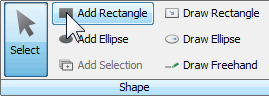
1. In the Shape group on the Analysis tab, click Add Rectangle.
2. Click each band to be analyzed, and an appropriately sized shape will be added around the band.
  
  For help choosing the right background subtraction method, see licorbio.com/BgSubtractHelp.
Export the quantification data for your HKP.
1. Click Shapes to open the Shapes data table.
2. Select shape data, then copy and paste data into a spreadsheet.
  
  All data fields will be exported, but “Signal” is the field of interest for analysis.

Target Protein Quantification (800 nm)

Select and view the 800 nm channel image only.
Add shapes to bands.
1. In the Shape group on the Analysis tab, click Add Rectangle.
2. Click each band to be analyzed, and an appropriately sized shape will be added around the band.
  
  For help choosing the right background subtraction method, see licorbio.com/BgSubtractHelp.
Export the quantification data for your target.
1. Click Shapes to open the Shapes data table.
2. Select shape data, then copy and paste data into a spreadsheet.
  
  All data fields will be exported, but “Signal” is the field of interest for analysis.

Normalization Calculations and Analysis of Replicates

Replication is an important part of QWB analysis, and is used to confirm the validity of observed changes in protein levels. Biological and technical replicates are both important, but meet different needs (2, 3).

Biological replicates: Parallel measurements of biologically distinct samples, used to control for biological variation and examine the generalizability of an experimental observation.
Technical replicates: Repeated measurements used to establish the variability of a protocol or assay, and determine if an experimental effect is large enough to be reliably distinguished from the assay noise.

Technical replication can be performed by testing the sample multiple times on the same gel or membrane (intra-assay variation) or by testing the sample multiple times in several Western blot experiments. This procedure describes the normalization and analysis of technical replicates that were tested multiple times on the same membrane.

Empiria Studio® Software will perform these calculations automatically. Please continue to the Data Interpretation section.

Calculate the Lane Normalization Factor for Each Lane (HKP, 700 nm)

Prepare a spreadsheet that contains the HKP and target protein quantification data.

Using the HKP data from the normalization channel, calculate the Average (arithmetic mean), Standard Deviation, and % Coefficient of Variation (% CV) of the replicate samples.

“Average” formula in Excel = AVERAGE(rep 1, rep 2, ……)

Standard Deviation formula in Excel = STDEV(rep 1 value, rep 2 value, …..)

Percent coefficient of variation formula

HKP (700 nm)

Lane	Sample treatment	Replicate	700 nm signal	Average Signal	St Dev	CV
1	none	1	1,000	900	100	11%
2		2	800
3		3	900
4	UV	1	800	833	58	7%
5		2	900
6		3	800

Example values shown for illustration only.

Calculate the Lane Normalization Factor (LNF) for each lane.

Identify the lane with the highest signal for the HKP.

Use this value to calculate the Lane Normalization Factor for each lane.

Western blot HKP lane normalization factor formula

Lane	Sample treatment	Replicate	700 nm signal	Highest Signal	Lane Normalization factor
1	none	1	1,000	1,000	1
2		2	800	1,000	0.8
3		3	900	1,000	0.9
4	UV	1	800	1,000	0.8
5		2	900	1,000	0.9
6		3	800	1,000	0.8

Normalization factors must be calculated for each blot. Normalization factors and standard curves cannot be reused between blots.

Calculate the Normalized Target Protein Signals (800 nm)

Using the Target Protein data from the 800 nm channel, calculate the Average, Standard Deviation, and % Coefficient of Variation of the replicate samples.

Target protein (800 nm), not normalized

Lane	Sample treatment	Replicate	Target (800 nm)	Average Signal	St Dev	CV
1	none	1	650	600	50	8%
2		2	550
3		3	600
4	UV	1	450	477	25	5%
5		2	500
6		3	480

Example values shown for illustration only.

Calculate the Normalized Target Signal for each target band by applying the LNF for that lane.

Divide the Target Signal for each lane by the corresponding LNF.

Calculate the Average, Standard Deviation, and % Coefficient of Variation of the replicates.

Target protein (not normalized)				Normalization		Normalized to HKP
Lane	Sample treatment	Replicate	Target (800 nm)	LNF (HKP)	Apply LNF	Norm. Target	Average signal	St Dev	CV
1	none	1	650	1	650 / 1	650	668	19	3%
2		2	550	0.8	550 / 0.8	688
3		3	600	0.9	600 / 0.9	667
4	UV	1	450	0.8	450 / 0.8	563	573	24	4%
5		2	500	0.9	500 / 0.9	556
6		3	480	0.8	480 / 0.8	600

Data Interpretation

Use the normalized target protein values for relative comparison of samples.

In the example above, target protein level is 14% lower in UV-treated samples than in untreated samples.
% CV can be used to evaluate the robustness of QWB results, and determine if the magnitude of observed changes in target protein levels is large enough to be reliably distinguished from assay variability.
1. The percent coefficient of variation (% CV) describes the spread or variability of measured signals by expressing the standard deviation (SD) as a percent of the average value (arithmetic mean). Because % CV is independent of the mean and has no unit of measure, it can be used to compare the variability of data sets and indicate the precision and repeatability of an assay.
  - A low % CV value indicates low signal variability and high measurement precision.
  - A larger % CV indicates greater variation in signal and reduced precision
2. On a Western blot, a change in band intensity is meaningful only if its magnitude substantially exceeds the % CV.
  - Generally speaking, the magnitude of the reported change should be at least 2X greater than the % CV.
    
    Example: To report a 20% difference between samples (0.8-fold or 1.2-fold change in band intensity), a CV of 10% or less would be recommended for replicate samples.
    
    For a specific measurement, this threshold for the magnitude of change would correspond to the mean + 2 SD.
  - Faint bands or subtle changes in band intensity are more difficult to detect reliably. In these situations, QWB analysis requires more extensive replication and low % CV.
  - This is a general guideline only. Replication needs and data interpretation are specific to your experiment, and you may wish to consult a statistician.
Compare the % CV of Target Protein replicates before and after normalization.
1. Normalization should not greatly increase the % CV of replicate samples.
2. The purpose of normalization is to reduce the variability between replicate samples by correcting for lane-to-lane variation. A large increase in % CV after normalization of replicates is a warning sign that the normalization method is not sufficiently robust, and may be a source of experimental error.

References

1. Janes KA (2015) An analysis of critical factors for quantitative immunoblotting. Sci Signal. 8(371): rs2.

2. Robasky, K, Lewis NE, and Church GM. Nat. Rev. Genet. 15: 56–62 (2014). http://www.nature.com/nmeth/journal/v11/n9/pdf/nmeth.3091.pdf

3. Naegle K, Gough NR, and Yaffe MB. Sci Signal. 8:fs7 (2015). https://www.ncbi.nlm.nih.gov/pubmed/25852186